
Introduction
I am Jung from the GLB Business Unit, Lakehouse Section.
In this article, I will introduce how to use KX's PyKX to connect Databricks and KX.
We will perform verification using kdb Insights license of KX's product kdb+ on Databricks.
kdb+ is the world's fastest time-series database and analytics engine.
Please check the article for more details on KX's product.
Contents
Introduction to PyKX
PyKX is the first Python interface to the world's fastest time-series database, kdb+, and primarily utilizes the vector programming language q. PyKX takes a Python-first approach to integrate q/kdb+ with Python. It offers users the ability to efficiently query and analyze vast amounts of in-memory and on-disk time-series data.
- The description of PyKX is quoted from the following KX document. code.kx.com
The verification process is as follows.
Download kdb Insights license
Install PyKX
Using the kdb Insights license, import PyKX
Try using KX's q language
Try using Databricks' EDA function
Performance comparison between PyKX and Pandas
Verification
1. Download kdb Insights license
Download the kdb Insights license to use kdb+. The kdb Insights license allows a free trial of KX's kdb Insights Personal Edition for 12 months.
Once you input personal information on the mentioned page, the license will be sent to you via email.
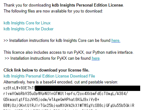
The license comes in two versions: one is a base64-encoded version written in the email, and the other is an LIC file version that is automatically installed when you click on "kdb Insights Personal Edition License Download File."
![]()
2. Install PyKX
Install PyKX on Databricks.
pip install pykx
3. Import PyKX
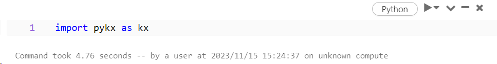
Use the kdb Insights license to import PyKX.
import pykx as kx
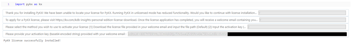
There are two methods to register the kdb Insights license.
➀This is a method to save the license file in the same location as the notebook. This can be done if the Python version is 3.10 or higher. It automatically loads the license.
➁This is a method for inputting the license. The instructions for inputting are available in the document below.
Those who have performed "1. Download kdb Insights license" can input Y / Y / 2 in order, then copy and input the license key received in the email, which will allow for the import.
4. Try using KX's q language.
Once you import PyKX, you can use KX's q language in Databricks' Python environment.
kx.q.til(10)
![]()
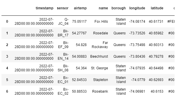
You can create a kdb+ table similar to a table in Databricks.
- After installing KX's public data (Time series) into Databricks, it can be loaded using pandas.
import pandas as pd
weather = pd.read_csv("自分のファイルのパス")
- Load the data from Databricks and import it into kdb+.
# Creating the same table into kdb+
kx.q["weather"] = weather
kx.q["weather"]
Let's try using KX's SQL.
kx.q.sql("SELECT * FROM weather limit 5")
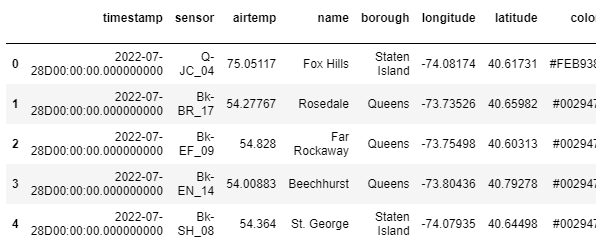
- Most of the features available in SQL can be used.
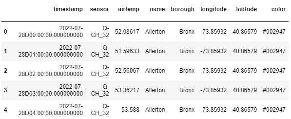
kx.q.sql("SELECT * FROM weather ORDER BY name limit 5")
kx.q.sql("SELECT * FROM weather WHERE borough = 'Staten Island' limit 5")
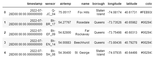
Load the data from kdb+ and convert it into a pandas table, then save it to Databricks as a CSV file.
# Creating the same table into pandas
df = kx.q["weather"].pd()
df.head(5)
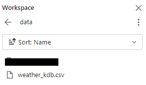
kx.q.write.csv('path_to_save/weather_kdb.csv', df)
![]()
5. Try using Databricks' EDA function
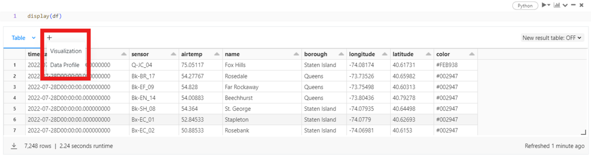
Databricks allows for simple exploratory data analysis (EDA) using features within the workspace. It loads data from kdb+ and visualizes it within Databricks.
display(df)
【+】When you press the button, Visualization and Data Profile appear.
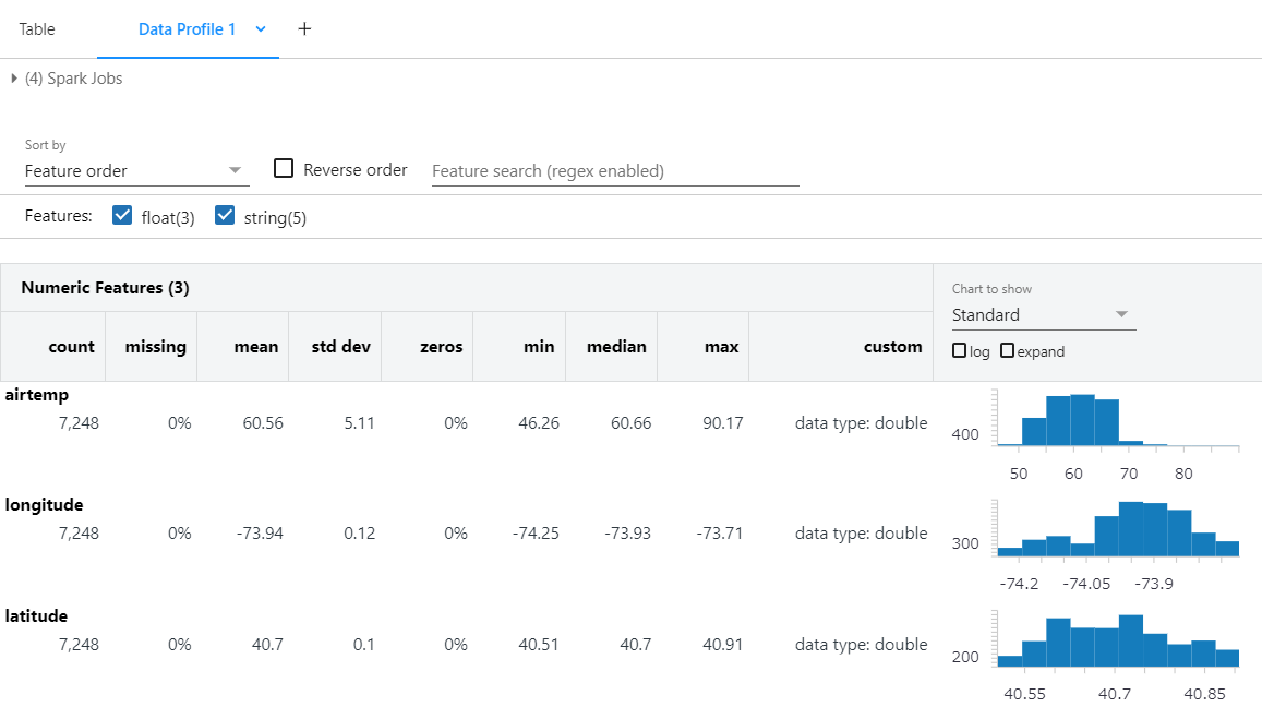
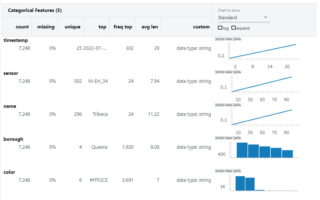
When using Data Profile, you can easily explore the characteristics of features. It classifies and displays them into Numeric Features and Categorical Features.
Numeric Features allow you to see missing values, basic statistics, and simple graphs.
In Categorical Features, you can easily see the number of unique values and the most frequent variables with their frequency count.
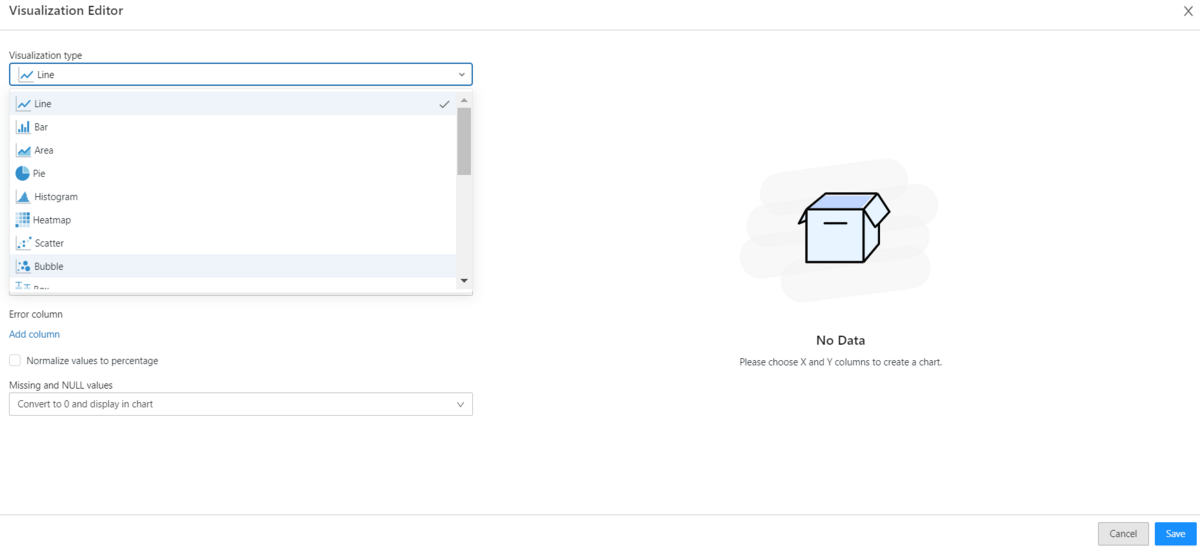
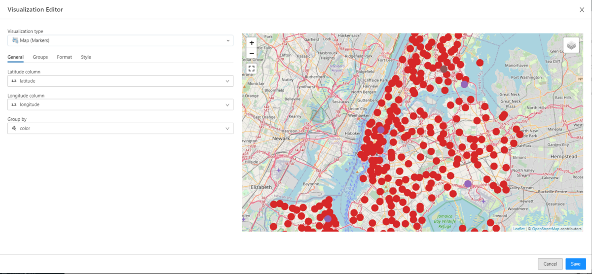
When using Visualization, you can visually create without coding using the UI.
You can select various types of charts using the dropdown.
* Please refer to the following URL for more details on the types of graphs.
- If you have longitude and latitude, mapping is possible.
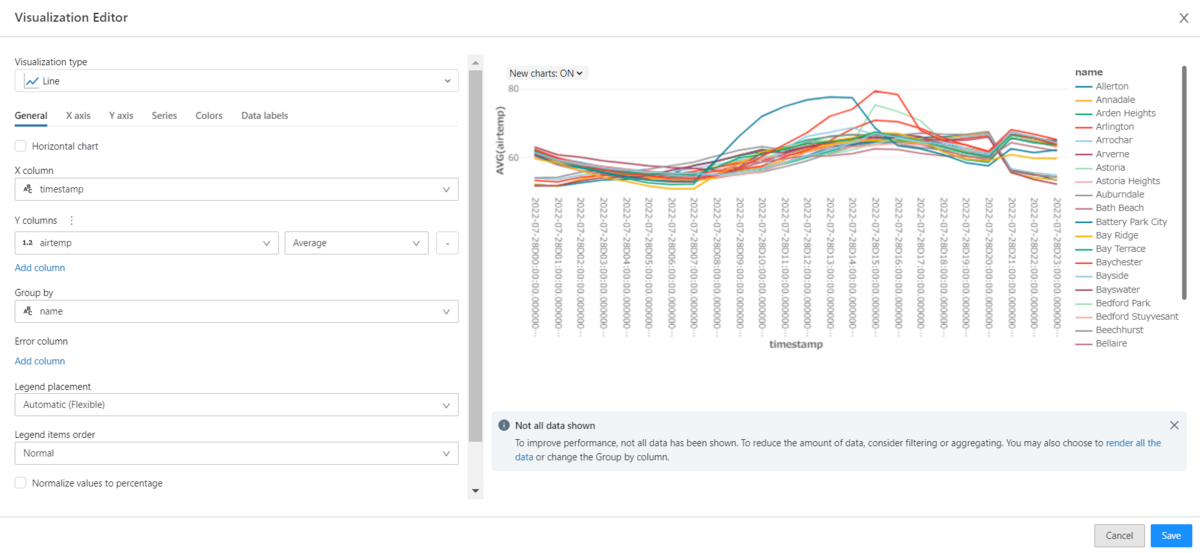
- Line graphs can be easily created through column settings (columns like X, Y, Group by, etc.).
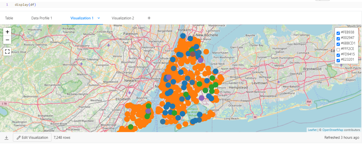
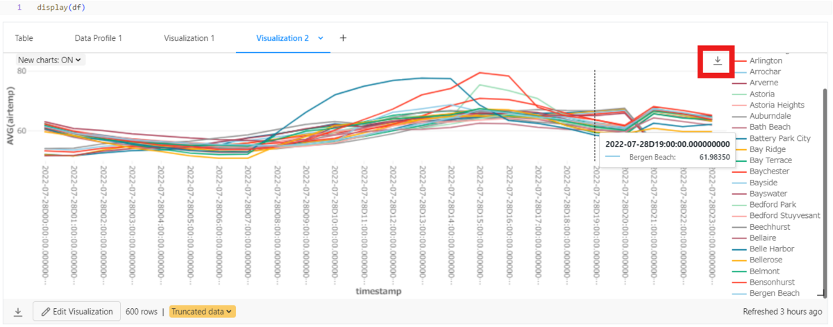
You can review the created graphs in the workspace.
- The layers of the map can also be adjusted in the workspace.
- You can save Line graphs as PNG files for images.
6. Performance comparison between PyKX and Pandas
Compare the performance of PyKX and Pandas.
The method of comparison was based on the materials below.
- Comparison of aggregation speed between kdb+'s q language and Pandas:
- Speed comparison and visualization of PyKX and Pandas:
Read the data using both PyKX and Pandas' csv read functionality. If you read the csv file with PyKX, it will be saved as a PyKX table, If read with Pandas, it will be saved as a Pandas data frame.
- Using PyKX
weather = kx.q.read.csv("自分のファイルのパス")
type (weather)
![]()
- Using PyKX
weather_pd = pd.read_csv("自分のファイルのパス")
type (weather_pd)
![]()
Check the column type of your data. If you read the data with Pandas, it may recognize timestamp as another type. If the type is not timestamp, you cannot use time-related functions such as date and time. If you need a Pandas data frame, you can use timestamp by reading the data with Pykx and converting the table to PD with Pykx.
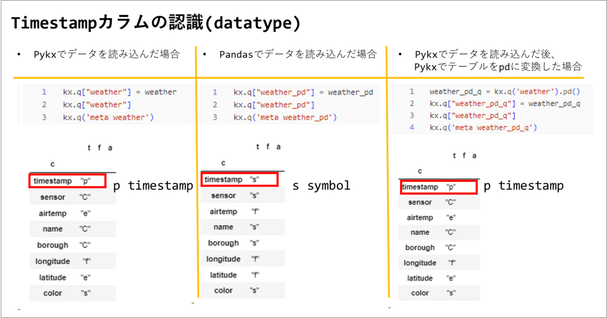
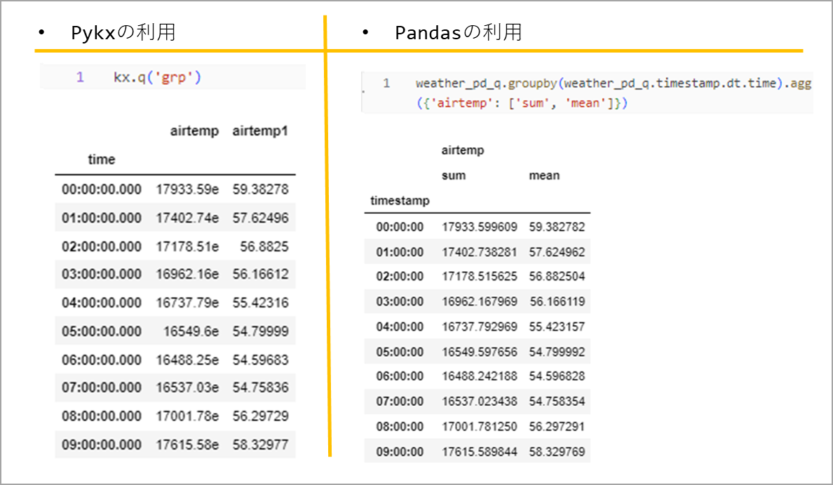
Compare the performance based on the time it takes when calculating sum and avg based on timestamp time. timestamp has the same format as "2022.07.28D00:00:00.000000000". The aggregation results will create a table like the one below.
When calculating 100 time series aggregations, use "%%capture" and "%timeit -n 100" to save the time taken in each variable.
- Using PyKX
%%capture pykx_time_res #Save the code result
%timeit -n 100 kx.q('grp:select sum airtemp, avg airtemp by timestamp.time from weather') #Measure the time it takes to calculate number 100
- Using Pandas
%%capture pandas_time_res #Save the code result
%timeit -n 100 grp=weather_pd_q.groupby(weather_pd_q.timestamp.dt.time).agg({'airtemp': ['sum', 'mean']}) #Measure the time it takes to calculate number 100
Create a function to use for visualization. For the function, I used a function from KX Academy. Some of the code was modified and used for this verification.
- ➀ String Processing Functions
# ➀ String Processing Functions
def fix_res_string(v) -> str:
    return v.stdout.split("\n")[0].replace("+-", "±")
- ➁ Function to dictionary input value to Pandas and PyKX
# ➁ Function to dictionary input value to Pandas and PyKX
def create_res_dict(pandas_time_res, pykx_time_res) -> pd.DataFrame:
    return pd.DataFrame(
        {
            "Time": {
                "Pandas": fix_res_string(pandas_time_res),
                "PyKX": fix_res_string(pykx_time_res),
            }
        }
    )
- ③ A function that converts the input dictionary into a data frame
# ③ A function that converts the input dictionary into a data frame
def parse_time_vals(d: dict) -> pd.DataFrame:
    all_rows = pd.DataFrame()
    for k, v in d.items():

        if "±" not in v:
            one_row = pd.DataFrame(
                {"avg_time": "", "avg_dev": "", "runs": "", "loops": ""}, index=[k]
            )

        else:
            avg_time, rest1, rest2 = v.split(" ± ")
            avg_dev, _ = rest1.split(" per loop")
            rest2 = rest2.strip(" std. dev. of ")
            rest2 = rest2.strip(" loops each)")
            runs, loops = rest2.split(" runs, ")
            one_row = pd.DataFrame(
                {"avg_time": avg_time, "avg_dev": avg_dev, "runs": runs, "loops": loops}, index=[k]
            )

        all_rows = pd.concat([all_rows, one_row])

    return all_rows.reset_index().rename(columns={"index": "syntax"})
- ④ If you input the value measured with "%timeit-n 100", the function returns the data frame of the function ③ after calculating the functions ➀ and ➁.
# ④ If you input the value measured with "%timeit-n 100", the function returns the data frame of the function ③ after calculating the functions ➀ and ➁.
def parse_vals(pandas_time_res, pykx_time_res) -> tuple[pd.DataFrame]:
    res_df = create_res_dict(pandas_time_res, pykx_time_res)
    return parse_time_vals(dict(res_df["Time"]))
- ⑤ Function to compare data frames (PyKX/Pandas)
# ⑤ Function to compare data frames (PyKX/Pandas)
def compare(df: pd.DataFrame, metric: str, syntax1: str, syntax2: str) -> float:
    factor = float(df[df["syntax"] == syntax1][metric].values) / float(
        df[df["syntax"] == syntax2][metric].values
    )
    str_factor = f"{factor:,.2f} times less" if factor > 1 else f"{1/factor:,.2f} time more"
    print(
        color.BOLD
        + f"\nThe '{metric}' for '{syntax2}' is {str_factor} than '{syntax1}'.\n"
        + color.END
    )
    return factor
- ⑥ Function to convert time
# ⑥ Function to convert time
def fix_time(l: list[str]) -> list[int]:
    fixed_l = []
    for v in l:
        if v.endswith(" ns"):
            fixed_l.append(float(v.strip(" ns")) / 1000 / 1000)
        elif v.endswith(" µs"):
            fixed_l.append(float(v.strip(" µs")) / 1000)
        elif v.endswith(" us"):
            fixed_l.append(float(v.strip(" us")) / 1000)
        elif v.endswith(" ms"):
            fixed_l.append(float(v.strip(" ms")))
        elif v.endswith(" s"):
            fixed_l.append(float(v.strip(" s")) * 1000)
        elif "min " in v:
            mins, secs = v.split("min ")
            total_secs = (float(mins) * 60) + float(secs.strip(" s"))
            fixed_l.append(total_secs * 1000)
        else:
            fixed_l.append(v)

    return fixed_l
- ⑦ Function to visualize
from tabulate import tabulate
import matplotlib.pyplot as plt
# ⑦ Function to visualize
def graph_time_data(df_to_graph: pd.DataFrame) -> pd.DataFrame:
    print(tabulate(df_to_graph, headers="keys", tablefmt="psql"))

    fig, ax = plt.subplots(figsize=(7, 3))

    df = df_to_graph.copy()
    df["avg_time"] = fix_time(df["avg_time"])
    df["avg_dev"] = fix_time(df["avg_dev"])
    df["upper_dev"] = df["avg_time"] + df["avg_dev"]
    df["lower_dev"] = df["avg_time"] - df["avg_dev"]

    _ = compare(df, "avg_time", "Pandas", "PyKX")

    df.plot(ax=ax, kind="bar", x="syntax", y="avg_time", rot=0)
    # df.plot(ax=ax, kind="scatter", x="syntax", y="upper_dev", color="yellow")
    # df.plot(ax=ax, kind="scatter", x="syntax", y="lower_dev", color="orange")

    ax.set_title("Pandas VS Pykx Time Taken")
    ax.set_ylabel("Average Time (ms)")
    ax.get_legend().remove()
    ax.set(xlabel=None)

    plt.show()

    return df
- Creating a class color
# Creating a class color
class color:
    PURPLE = "\033[95m"
    CYAN = "\033[96m"
    DARKCYAN = "\033[36m"
    BLUE = "\033[94m"
    GREEN = "\033[92m"
    YELLOW = "\033[93m"
    RED = "\033[91m"
    BOLD = "\033[1m"
    UNDERLINE = "\033[4m"
    END = "\033[0m"
Visualize using the function you created. When aggregating using timestamps, pykx was found to be 11.7 times faster than pandas.
time_res_df = parse_vals(
    pandas_time_res, pykx_time_res
)

numeric_time_res_df = graph_time_data(time_res_df)
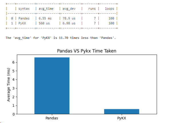
For time series analysis, PyKX gave better results in terms of use of timestamp type and aggregation speed.
Summary
In this post, I registered the kdb Insights license on Databricks and tried using KX's kdb. By using a library called PyKX, it's possible to access KX's KDB from Python and use the q language. This is recommended for those who want to utilize both the functionalities of Databricks and KX's KDB+.
Thank you for reading until the end.
Your continued support is greatly appreciated!

We offer comprehensive support, from implementing data analysis infrastructure using Databricks to aiding in internalization. If you're interested, please feel free to contact us.
Also, we are currently recruiting individuals who can work with us! We look forward to hearing from those who are interested in APC.
Translated by Johann