
Introduction
This is Abe from the Lakehouse Department of the GLB Division. In this article, we will introduce a method to search for images similar to head MRI images using KDB.AI.
KDB.AI is a knowledge base vector database and search engine provided by KX systems. Vector databases can analyze and process vast amounts of text data, and by converting text data into vector format, computers can understand and respond to natural language input. Developers can build scalable and reliable real-time applications by using real-time data to provide advanced search, recommendations, and personalization for AI applications.
An overview of KDB.AI and explanations about account creation are explained in the previous article.
In this article, we will introduce a method to save a brain MRI image as a vector in KDB.AI and search for images similar to that image. It is also created based on the sample code provided by KDB.
- Introduction
- Purpose of the Tutorial
- Preparation
- 1. Load Image Data
- 2.Create Image Vector Embeddings
- 3. Store Embeddings in KDB.AI
- 4. Query KDB.AI Table
- 5. Search For Similar Images To A Target Image
- 6. Delete the KDB.AI Table
- Conclusion
Purpose of the Tutorial
The purpose of this tutorial is to show you how to create an embedding using a trained neural network and save it to a vector database. You will also learn how to use KDB.AI to find similar images to the input image. Specifically, follow the steps below.
- Loading image data
- Creating an embedding image
- Saving embedding images to KDB.AI
- Querying KDB.AI tables
- Similar image search for target image
- Delete KDB.AI table
The code in this article is taken from the GitHub repository.
The execution environment is a Databricks workspace, but you can run it with your favorite editor.
Preparation
Now let's take a look at the code. First, install the necessary packages and restart the Python process.
pip install huggingface_hub umap-learn hdbscan tensorflow Pillow matplotlib kdbai_client -q
dbutils.library.restartPython()
Import the required Library.
# download data
import os
from zipfile import ZipFile

# embeddings
from tensorflow.keras.applications.resnet50 import ResNet50, preprocess_input
from tensorflow.keras.preprocessing import image
from PIL import Image
import numpy as np
import pandas as pd
import ast

# timing
# A library that displays the progress of loops and iterable operations as a progress bar.
from tqdm.auto import tqdm

# vector DB
import kdbai_client as kdbai
#Provides utilities to securely enter sensitive information like passwords without displaying them
from getpass import getpass
import time

# plotting
import hdbscan
import umap.umap_ as umap
from matplotlib import pyplot as plt
You may get a warning 'Could not find TensorRT', but ignore it as it will not affect later code.
Let's also define a Helper Function in advance.
# Check the shape and contents of the DataFrame
def show_df(df: pd.DataFrame) -> pd.DataFrame:
    print(df.shape)
    return df.head()

# Load and display images
def plot_image(axis, source: str, label=None) -> None:
    axis.imshow(plt.imread(source))
    axis.axis("off")
    title = (f"{label}: " if label else "") + source.split("/")[-1]
    axis.set_title(title)
1. Load Image Data
The sample dataset used is a brain tumor classification image obtained from Kaggle. The dataset consists of MRI brain scan images organized into four classes (glioma, melanoma, pituitaryoma, no tumor) based on the brain tumor in the image.
The original Kaggle dataset consists of two folders, a Training folder and a Testing folder, both of which contain images organized by tumor class. These images were preprocessed by resizing them to (224, 224, 3), renaming each image's class, and giving each image a unique ID within the directory.
After preprocessing, the dataset's Training folder is used to train a ResNet model, which we will use during embedding. After processing, the Testing folder will be renamed to data and will be used in this notebook. Of course, the ResNet model is not learning the test data in the Testing folder, which helps avoid overfitting when creating the embedding.
Define List Of Paths To The Extracted Image Files
Next, extract the image file paths from different subfolders within the 'Testing' directory. We need these to pass to the function that creates the embedding later.
def extact_file_paths_from_folder(parent_dir: str) -> dict:
    image_paths = {}
    for sub_folder in os.listdir(parent_dir):
        sub_dir = os.path.join(parent_dir, sub_folder)
        image_paths[sub_folder] = [
            os.path.join(sub_dir, file) for file in os.listdir(sub_dir)
        ]
    return image_paths
image_paths_map = extact_file_paths_from_folder("data")
You can see that we were able to get the path of the image file.
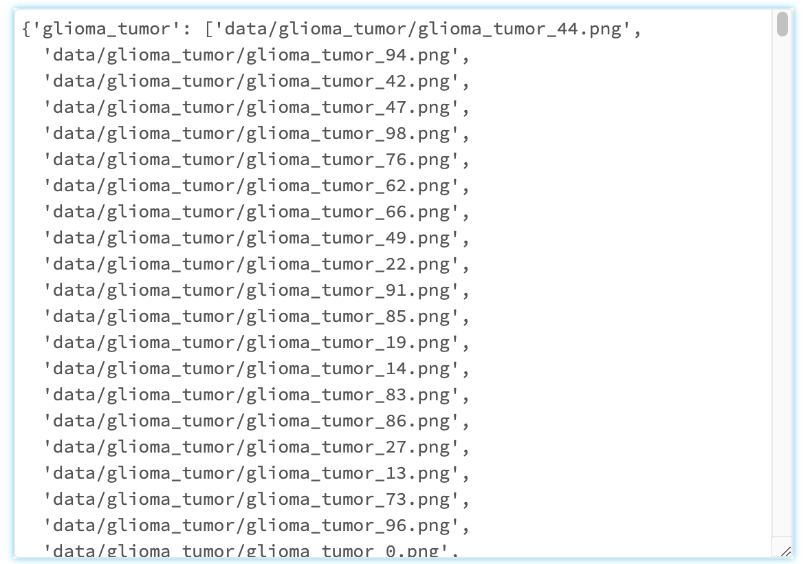
Image files are numbered from 1 to 100, and images can be retrieved from each folder.
Next, use the plot_image() helper function to display image number 20 as an example.
image_index = 20  # feel free to change this!

# create subplots
_, ax = plt.subplots(nrows=len(image_paths_map) // 2, ncols=2, figsize=(10, 8))
axes = ax.reshape(-1)

# get image at specified index
for i, (_, image_paths) in enumerate(image_paths_map.items()):
    for path in image_paths:
        if path.endswith(f"{image_index}.png"):
            break

    # plot each image in subplots
    plot_image(axes[i], path)
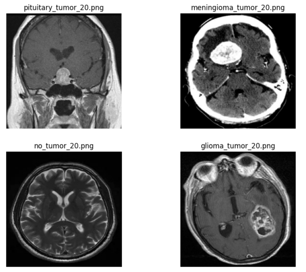
Images could be displayed for each tumor class.
Load data using image_dataset_from_directory()
The image_dataset_from_directory() function has been imported from TensorFlow's Keras API, and is a function that efficiently handles image data during deep learning training and evaluation. It stores each image with its corresponding class label in that image's directory, so you can retrieve the data and its label in a format suitable for embedding.
dataset = image_dataset_from_directory(
    "data",
    labels="inferred",# Label inferred from directory name
    label_mode="categorical",# Get labels in one-hot encoding format
    shuffle=False,
    seed=1,
    image_size=(224, 224),
    batch_size=1,
)
2.Create Image Vector Embeddings
We use a trained neural network for brain tumor classification to create image embeddings. This example uses a network with a ResNet-50 backbone. ResNet-50 is a neural network architecture commonly used for general image classification tasks.
ResNet-50 was originally trained on the ImageNet dataset, and the dataset does not include MRI images. Examples of different brain tumor images are not included, so ResNet-50 is retrained to classify MRI brain scan images.
Load Pre-Trained Classification Neural Network
Load a model to classify MRI images. Load the retrained model called mri_resnet_model from KX from Hugging Face Hub.
model = from_pretrained_keras("KxSystems/mri_resnet_model")
Check the structure of the model.
model.summary()
_________________________________________________________________
 Layer (type)                Output Shape              Param #
=================================================================
 resnet50 (Functional)       (None, 2048)              23587712

 flatten_1 (Flatten)         (None, 2048)              0

 dense_2 (Dense)             (None, 8)                 16392

 dense_3 (Dense)             (None, 4)                 36

=================================================================
Total params: 23604140 (90.04 MB)
Trainable params: 23551020 (89.84 MB)
Non-trainable params: 53120 (207.50 KB)
_________________________________________________________________
This model consists of four layers (ResNet-50, Flatten, and two Dense), and the ResNet-50 layer is actually an abstraction of many layers under one name. , contains millions of parameters. The Flatten layer flattens the output of ResNet-50 into a (1, 2048) vector (feature vector), and the last two Dense layers (or fully connected layers) convert the ResNet-50 feature vector to the input image. Convert to 4 columns of data according to the class.
The network diagram below details the results of model.summary().
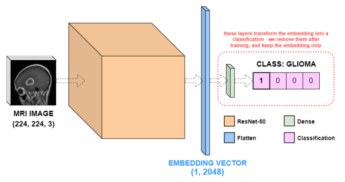
(Retrieved from https://github.com/KxSystems/kdbai-samples/blob/main/image_search/image_search.ipynb)
Transform Classification Network Into Embedding Network
Dense layers were needed to classify the four brain tumor classes, but they are no longer needed. In this example, we are not interested in the output value of the Dense layer, but the value after embedding. Therefore, call pop() to remove the two Dense layers in the above model. The new output of the model is a (1, 2048) feature vector, i.e. a ResNet-50 embedding vector of the input image.
model.pop()
model.pop()
model.summary()
_________________________________________________________________
 Layer (type)                Output Shape              Param #
=================================================================
 resnet50 (Functional)       (None, 2048)              23587712

 flatten_1 (Flatten)         (None, 2048)              0

=================================================================
Total params: 23587712 (89.98 MB)
Trainable params: 23534592 (89.78 MB)
Non-trainable params: 53120 (207.50 KB)
_________________________________________________________________
I was able to remove the Dense layer.
Use Embedding Network To Create Image Embeddings
To obtain embedding data, we use a model to extract features for each image, and then save the features and class labels in respective Numpy arrays.
# create empty arrays to store the embeddings and labels
num_files = len(dataset)
embeddings = np.empty([num_files, 1, 2048])
labels = np.empty([num_files, 1, 4])

# for each image in dataset, get its embedding and class label
for i, image in tqdm(enumerate(dataset)):
    embeddings[i, :, :] = model.predict(image[0], verbose=0)
    labels[i, :, :] = image[1]
Now that we have the class labels, we can get the tumor type by checking which index in the vector is equal to 1.
# reduce these vectors from 3 dimensions to 2 dimensions
reduced_embeddings = embeddings[:, 0, :]
reduced_labels = labels[:, 0, :]

# list the tumor types in order
tumor_types = ["glioma", "meningioma", "no_tumor", "pituitary"]

# for each vector, save the tumor type given by the high index
class_labels = [tumor_types[label.argmax()] for label in reduced_labels]
It's often useful to store the entire file path rather than just the name of the image, so in the cell below I iterate through the files and store the file path.
# get a single list of all paths
all_paths = []
for _, image_paths in image_paths_map.items():
    all_paths += image_paths

# sort the source_files in alphanumeric order
sorted_all_paths = sorted(all_paths)
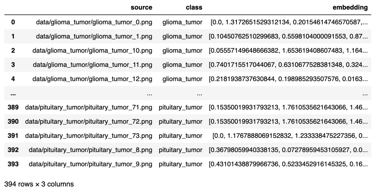
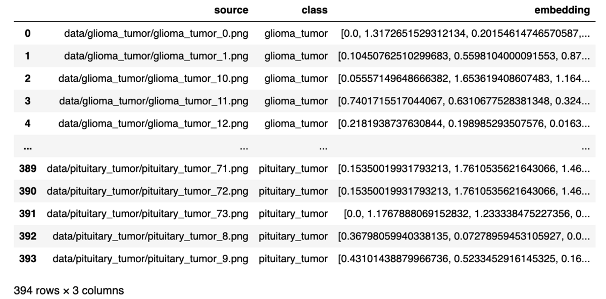
Now we have all the components: image file path, image class, and vector embedding. The next step is to convert everything to a DataFrame for insertion into KDB.AI's vector database.
embedded_df = pd.DataFrame(
    {
        "source": sorted_all_paths,
        "class": class_labels,
        "embedding": reduced_embeddings.tolist(),
    }
)

show_df(embedded_df)
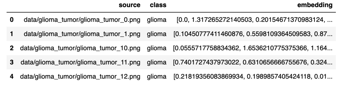
We have created a DataFrame consisting of the image file path, tumor class, and embedding values.
Visualising The Embeddings
Since the embedding of features is high-dimensional, it is difficult to understand how they can be organized and clustered. UMAP is an easy-to-understand way to recognize feature organization. UMAP is a method of dimensionality reduction and a technique for visualizing clustering in 2D. This not only provides a better understanding of the success of the classification network, but also provides insight into where misclassifications may occur.
_umap = umap.UMAP(n_neighbors=15, min_dist=0.0) # UMAP's instance
umap_df = pd.DataFrame(_umap.fit_transform(reduced_embeddings), columns=["u0", "u1"]) # dimensionality reduction
Indicates the parameters when creating a UMAP instance.
- n_neighbors``: Specifies how much UMAP considers each data point's neighbors. Larger values emphasize global data structures; lower values emphasize local data structures.
-min_dist``: Specifies the minimum distance between data points in low-dimensional space. When this distance is small, the data points tend to form clusters; when it is large, the data points tend to spread out.
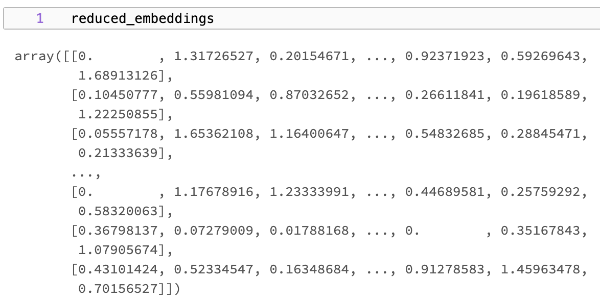
Before dimension reduction
reduced_embeddings
After dimension reduction
show_df(umap_df)
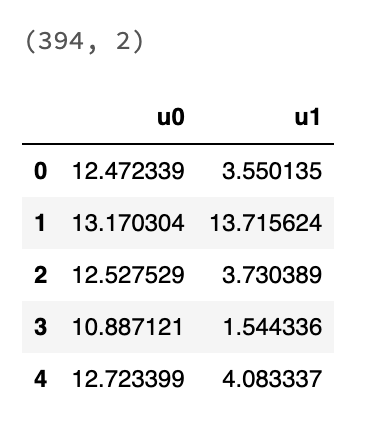
I was able to reduce the dimensionality to a 2D DataFrame using UMAP.
Next, cluster the dimensionally reduced embedding data. HDBSCAN (Hierarchical Density-Based Spatial Clustering of Applications with Noise) is used for clustering.
_hdbscan = hdbscan.HDBSCAN(min_cluster_size=5)
clusters = _hdbscan.fit_predict(umap_df)

# number of unique clusters
len(list(set(clusters)))
22
22 clusters were formed. min_cluster_size specifies the minimum number of points to be recognized as a cluster. In this example, clusters with fewer than 5 points are treated as noise.
Now plot the embedding in 2D, displaying each class in a different color.
# define color for each class label
class_colors = {
    'glioma': 'blue',
    'meningioma': 'red',
    'no_tumor': 'green',
    'pituitary': 'purple',
}

# Create a figure for plotting
plt.figure(figsize=(10, 8))

# Scatter plot with 'u0' and 'u1' columns as x and y, color mapped by class_labels
for class_label, color in class_colors.items():
    indices = [i for i, label in enumerate(class_labels) if label == class_label]
    subset = umap_df.iloc[indices]
    plt.scatter(subset['u0'], subset['u1'], label=f'{class_label}', color=color)

# beutify plot
plt.title('Embeddings Map for MRI Brain Scan Images')
plt.xlabel('u0')
plt.ylabel('u1')
plt.legend()
plt.show()
This is the result of plotting embedding for each tumor class.
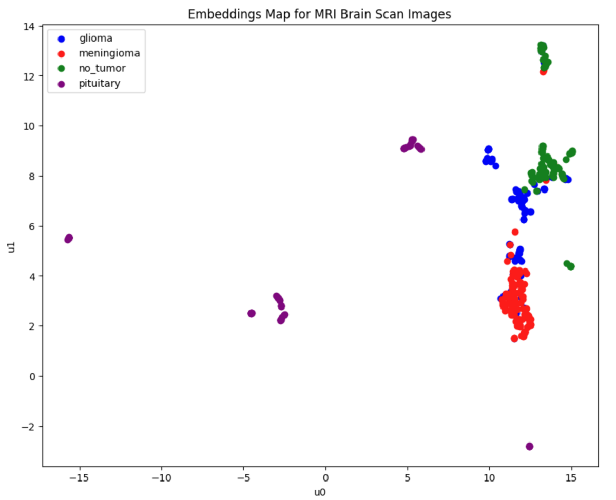
As shown above, most of the data can be separated between classes, but there is still some overlap, especially in the glioma class (shown in blue). However, for most of the points on the graph, the "nearest point" belongs to the same class as yourself. Therefore, when performing a vector similarity search using embedding data, the majority of results should be of the same class.
3. Store Embeddings in KDB.AI
Connect to the KDB.AI session. To use KDB.AI, you need two pieces of session information: a URL endpoint and an API key. You can sign up for free here.
Connect to the KDB.AI session from `kdbai.Session and pass the session URL endpoint and API key details from the KDB.AI cloud portal.
KDBAI_ENDPOINT = (
    os.environ["KDBAI_ENDPOINT"]
    if "KDBAI_ENDPOINT" in os.environ
    else input("KDB.AI endpoint: ")
)
KDBAI_API_KEY = (
    os.environ["KDBAI_API_KEY"]
    if "KDBAI_API_KEY" in os.environ
    else getpass("KDB.AI API key: ")
)
Create a session.
session = kdbai.Session(api_key=KDBAI_API_KEY, endpoint=KDBAI_ENDPOINT)
Define Vector DB Table Schema
Define the schema for the KDB.AI table that will store the embedded data. This table contains the same three columns as the embedding dataframe:
source: File path to raw image file
class: Tumor class label
embedding:2048-dimensional feature vector for similarity search
image_schema = {
    "columns": [
        {"name": "source", "pytype": "str"},
        {"name": "class", "pytype": "str"},
        {
            "name": "embedding",
            "vectorIndex": {"dims": 2048, "metric": "L2", "type": "hnsw"},
        },
    ]
}
Crate Vector DB Table
Next, use the KDB.AI create_table() function to create a table that matches the schema defined in the Vector database.
# ensure the table does not already exist
try:
    session.table("mri").drop()
    time.sleep(5)
except kdbai.KDBAIException:
    pass

table = session.create_table("mri", image_schema)
Add Embedded Data to KDB.AI Table
Check the memory usage of your data before inserting it into KDB.AI. This is because the recommended data size is 10MB or less.
# convert bytes to MB
embedded_df.memory_usage(deep=True).sum() / (1024**2)
If it's larger than 10MB, I would consider batch (chunk) splitting, but since this dataset is only 6MB, I can insert all the data at once.
table.insert(embedded_df)
Verify Data Has Been Inserted
If you run table.query(), you will see that the data has been added.
table.query()
4. Query KDB.AI Table
Now that all image embeddings are registered in KDB.AI's database, we are ready to demonstrate KDB.AI's fast query capabilities.
Query functions accept a variety of arguments for easy filtering, aggregation, and sorting. You can see all of this by running table.query().
Let's demonstrate this by filtering for images with "glioma" in the file name.
table.query(filter=[("like", "class", "*glioma*")])
We were able to obtain the data source and embedding data whose tumor class is "glioma".
5. Search For Similar Images To A Target Image
Finally, we perform an image similarity search. This is done using the table.search() function.
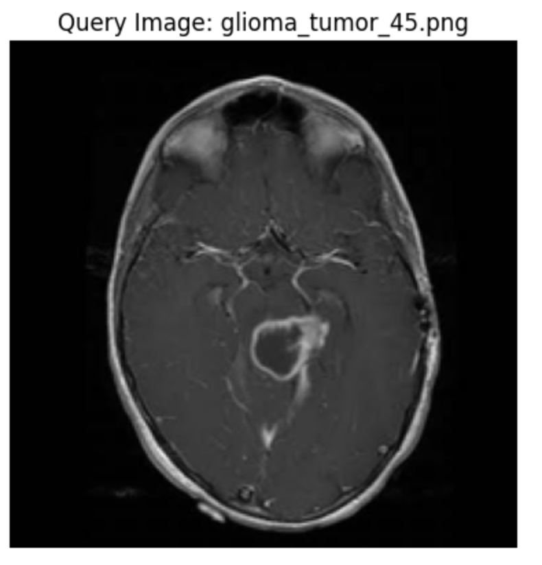
Choose Example Image
First, randomly select a row from the test dataset.
# Get a sample row
random_row_index_1 = 40

# Select the random row and the desired column's value
random_row_1 = embedded_df.iloc[random_row_index_1]

plot_image(plt.subplots()[-1], random_row_1["source"], label="Query Image")
Search for similar images to this image.
Save the embedding of this image in the sample embedding variable.
sample_embedding_1 = random_row_1["embedding"]
Search Based On The Chosen Image
Using the embedding data extracted with sample_embedding, find the eight neighboring images closest to the query image.
results_1 = table.search([sample_embedding_1], n=8)
results_1[0]
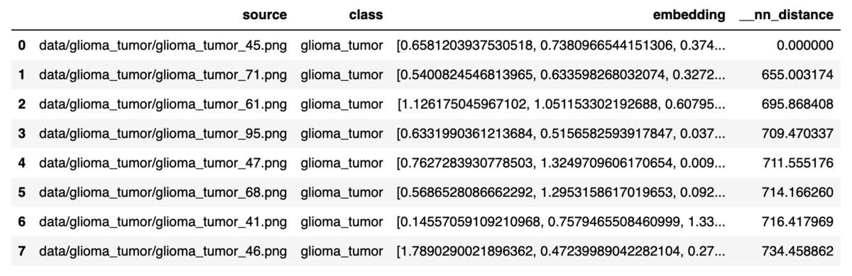
The results returned from table.search() will display the closest match along with the value of the nearest neighbor distance __nn_distance. Of course, __nn_distance from the sample image selected earlier will be 0.
Plot Most Similar Images
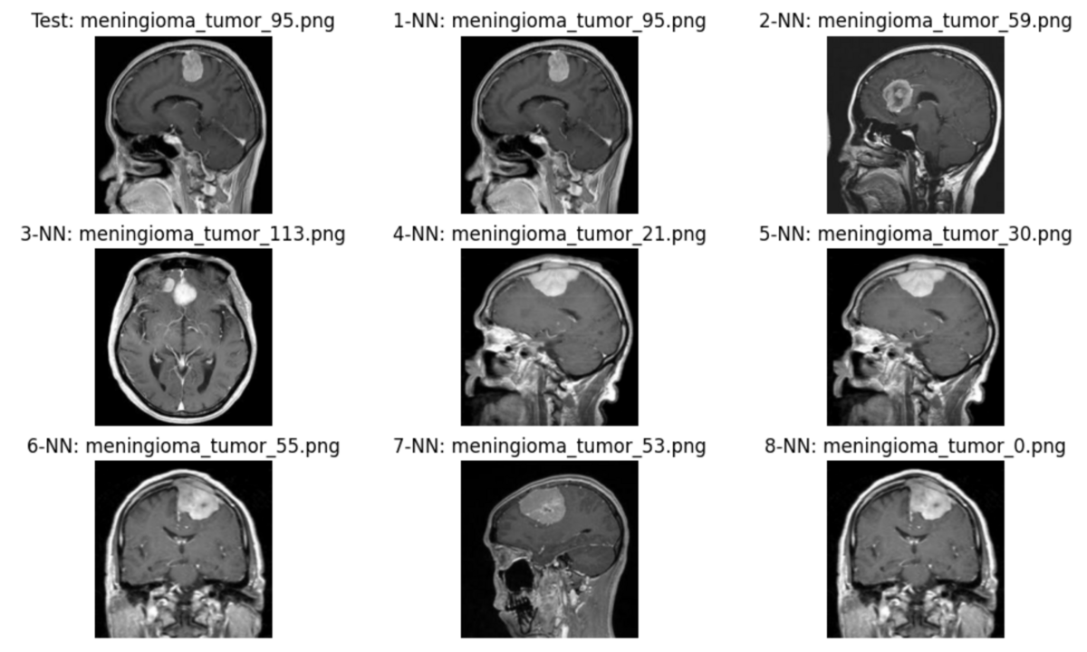
Let's visualize these images. The plot_test_result_with_8NN() function plots the query image and its eight nearest neighbors.
def plot_test_result_with_8NN(test_file: str, neighbors: pd.Series) -> None:
    # create figure
    _, ax = plt.subplots(nrows=3, ncols=3, figsize=(12, 7))
    axes = ax.reshape(-1)

    # plot query image
    plot_image(axes[0], test_file, "Test")

    # plot nearest neighbors
    for i, (_, value) in enumerate(neighbors.items(), start=1):
        plot_image(axes[i], value, f"{i}-NN")

nn1_filenames = results_1[0]["source"]
plot_test_result_with_8NN(random_row_1["source"], nn1_filenames)
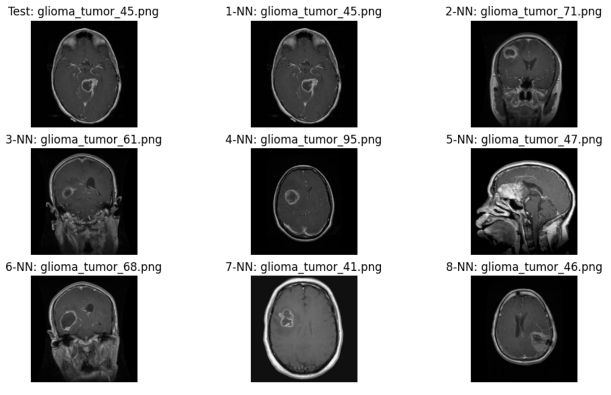
Although some of the images returned are from different cross-sections, I believe the contrast of the tumor is similar to the test image.
Automate This Search Process
Based on the above steps, we will define the process from selecting a sample image to displaying 8 images as the mri_image_nn_search function.
def mri_image_nn_search(table, df: pd.DataFrame, row_index: int) -> None:
    # Select the random row and the desired column's value
    row = df.iloc[row_index]

    # get the embedding from this row
    row_embedding = row["embedding"]

    # search for 8 nearest neighbors
    nn_results = table.search([row_embedding], n=8)

    # plot the neighbors
    plot_test_result_with_8NN(row["source"], nn_results[0]["source"])
Find similar images with another sample image.
# Get another row
random_row_index_2 = 210

mri_image_nn_search(table, embedded_df, random_row_index_2)
The cross-sectional images of the returned similar image and the test image are different, but I think the contrast of the tumor is similar. I believe that these results will provide diagnostic material for doctors to determine whether or not it is a tumor.
6. Delete the KDB.AI Table
This completes the process from preparing the dataset to searching for images similar to the test image. It is a best practice to throw away a table when you are finished using it.
table.drop()
Conclusion
In this article, we performed a similar search for MRI images using KDB.AI. This time, we focused on MRI images, but since KDB.AI has a high-speed query function, I think it can also be used for real-time defective product detection on manufacturing lines.

The Lakehouse department is looking for an engineer/PM to perform development and consulting on data & AI projects. We are also recruiting in other departments, so if you are interested in APC, please contact us for a casual interview (Job Listing).
Translated by Johann